
Potential GDP is widely used in quantitative (quant) and other investment models that select investments (such as sector rotations) based on what an economy is capable of producing if resources were more fully used. As it is a rather mysterious bit of math, investors often just take it as a given. Yet, because it glues together so many assumptions, investors would do well to poke on it. With a fresh look, Potential GDP is higher than generally assumed mostly because more resources are available and inflation pressures are lower. Inflation pressures are lower because a) the official unemployment rate doesn’t fully reflect available labor and b) trends show consumers are able to buy more at lower prices. This insight creates opportunity for investors. For individual investors who simply reference Potential GDP for cycle strategies; lower the weighting or shift to another strategy. For quants designing models, reset your models.
Just so you know… This is intended for modelers or individual investors with “inquiring minds.” Thus, some background is assumed. Hyperlinks are provided to related Fed Dashboard & Fundamentals articles and other sources. For academics, apologies that this breezes over hot topics in math and theory. Here, emphasis is modestly on illuminating data trends for investors. If you would like just a few more bullets, then skip to the end and read the “Bottom line for investors.”
Still reading? Great – enjoy the mysteries revealed and have fun investing better…
An investor’s questions are, “How well does Potential Gross Domestic Product (GDP) measure what it says it measures – what an economy is capable of producing?” “Have dynamics changed over time in a way that isn’t fully reflected in today’s measure?” And, if so, “What is it really?”
To be on the same page, we start by clarifying “Potential GDP.” It is not maximum or national emergency output. It is usually defined as the level of output (“real” or price-level adjusted) that can be sustained over time without fostering inflation (general price level from money, rather than from product supply and demand causes).
A widely used calculation of Potential GDP is labor and capital inputs multiplied by productivity. “Capital” means physical capital — equipment, buildings and intellectual property products. “Productivity” in the more inclusive calculations is “Total Factor Productivity” (TFP) more modestly known as “Multifactor Productivity” (MFP) as described previously. It can also be single factor calculations, usually labor productivity.
With this in mind, let’s consider the capital and labor capacity available and what that implies about potential production (GDP) today.
Labor hours are more plentiful
- Hours worked is relatively straight-forward, published by the U.S. Bureau of Labor Statistics (BLS) based on the Current Employment Statistics (CES) survey. Business Sector Hours Worked relative to Civilian noninstitutional population (age 16 and older) was on an uptrend from 1975 to 1999 and has been on a downtrend since. It is currently on a rebound from the credit bubble crash. Today, we’re working about 20% fewer hours per person than in 1974 and about 15% fewer than the 1999 peak. This happened while the number of people age 65 and over in the labor force more than doubled since 2000. Higher hours worked in the past point to more potential production today.
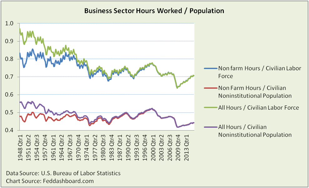
- Labor productivity is not directly measured. It is derived by dividing output by hours worked. Output is Real GDP provided by the U.S. Bureau of Economic Analysis (BEA). As the hours worked (denominator in the ratio) have been bouncing back, the labor productivity ratio has taken a hit as shown previously. Dynamics of hours worked and global trade were discussed in the story of the Red Dots. More on productivity after some comments on capital…
Physical capital is more plentiful
Physical Capital includes Structures, Equipment and Intellectual Property (IP) Products (including R&D, software and patents). Physical capital can be viewed similar to labor productivity, dividing output by each input. Pictured below is the current replacement cost of net stock; it’s a more basic view before assumptions are made about how the capital is used. As this is private capital data, the output is Private GDP (Business, Households and Nonprofits – excluding Government).
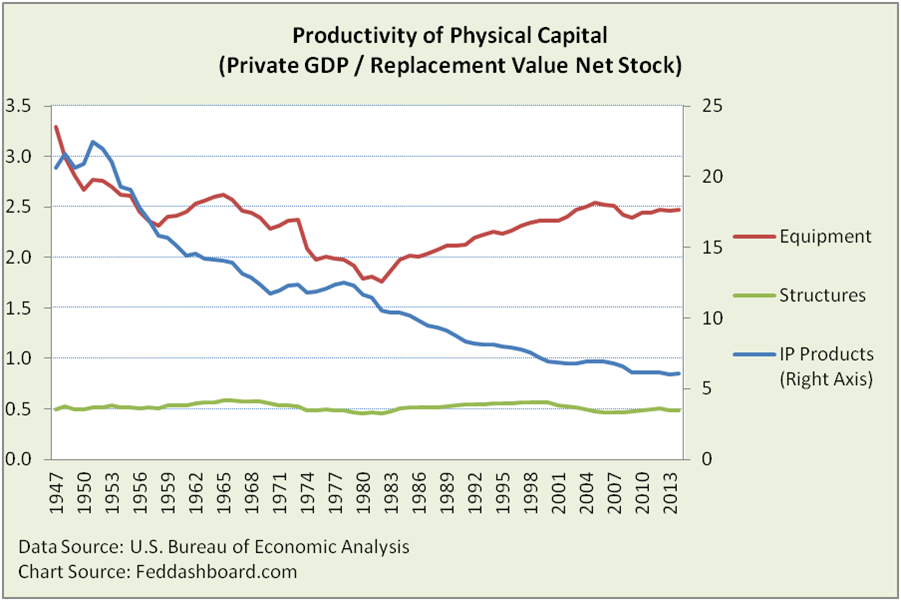
- IP Products productivity is plunging (notice the right hand scale) because the net stock is growing – if more is used, then it’s deemed less productive. A nuance in productivity math is that today’s “great idea” becomes tomorrow’s higher-bar. Why? Because when a productive idea gets formalized into software, research and development program, or patent, then it becomes part of the asset base that the next year’s idea must beat. So the faster ideas are formalized, the more measured productivity is penalized. There are many nuances of IP accounting that disconnect measured productivity from Henry Ford’s practical adage, “Work smarter, not harder.” Shifting from measurement to the substance of the innovation debate, innovation appears healthy for three reasons: 1) lab pipeline of tech is historically healthy, 2) the way tech pessimists value patents as number of citations isn’t reality, and 3) research-to-retail product price-quantity curves show persistent growth over past decades as illustrated in the Exponential Technology section.
- Equipment productivity is going up in this replacement (current) cost view. Is that because the net stock is less? No. It’s because prices are falling and/or quality is better. On a productivity historical cost book value basis, equipment has been on a downtrend (using more equipment) until about 1983 when it roughly stabilized. At the extreme, consider a $1 million gene sequencer from a few years ago that now sells for just $1 as equipment improves dramatically.
- Structures have been relatively flat in this net stock view. Manufacturing and most others industries have been declining. The Structure average has been helped by hospitals, education, mining (oil & gas) before the bust and information processing (data centers).
Another view emerges when physical capital is compared to hours worked. Here, Structures skyrocket as the ratio implies they are being used more “efficiently” per hour worked. In office buildings, this is observed in worker “hotel” or “bullpen” space, or work-at-home rather than individual offices. In manufacturing it is smaller footprint manufacturing, often with smaller equipment and less inventory storage.
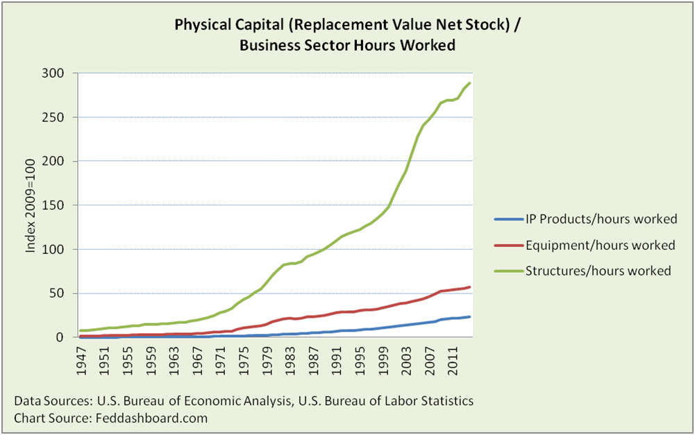 Notice Equipment and IP Products, recently slowing in growth reflecting hours worked increased as shown previously and utilization described in this note.
To make changes more clear for nonresidential structures and equipment, we flip the view to quarterly investment additions relative to Private GDP. Structures have been on a downtrend since the 1970s when manufacturing peaked.
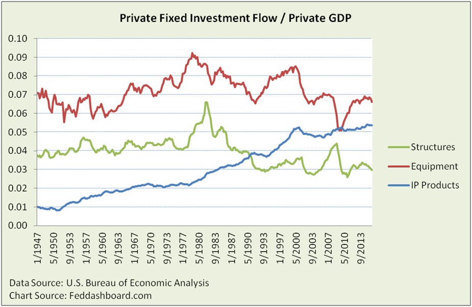
Less physical capital has been needed to produce than in past. This includes shift in industry composition and country sourcing. For Structures, the real fixed investment (not shown) has been flat since the mid 1970s with peaks in 1981, 1985, 2000 and 2008 – each about 20% higher than current levels. Higher investment in the past both reflects the need for less physical capital and points to higher potential production today.
Given these tangible changes, why isn’t Potential GDP higher?
Mystery revealed in measurement of timing and productivity
Timing is about: 1) the look back time range and 2) the prediction period.
- The look back period is the number of past years used as a reference for predicting the future. To avoid irrelevant history hurting predictions, the convention is to look back to the beginning of the most recent complete business cycle (2001) and then adjust for how the current cycle might play out. But, while solving one problem, this convention creates another by missing hours and capital available for potential production. These available resources, accumulated over the decades, are visible in people insufficiently working and production plants built for prior eras that today could hold more people and equipment. Skills are a constraint for some occupations. But, recall the high proportion of new jobs in low-skill occupations. In short, because available resources have been undercounted, potential production is higher.
- The prediction period is simply the year being predicted, such as 2019. Here, the convention is to limit potential output to capacity inputs that would be available in that period. This is most clear in how data for the current period are collected. The U.S. Census Bureau Plant Capacity Utilization survey defines maximum capacity as “production that this establishment could reasonably expect to attain under normal and realistic operating conditions fully utilizing the machinery and equipment in place.” This is not a bad definition. But, it is designed for a different purpose — to measure idle capacity. This is not what could be potentially manufactured, even in the same facility and same year by improving equipment or management methods. Further, production potential is greater because production methods have become more flexible. How flexible? Consider: 1) long plant shutdowns for retooling are a thing of the past, 2) many improvements are merely software upgrades, and 3) North Dakota Mining and Logging employment had 12 month increases of 74% or more for six months starting August 2010. In short, because 1) structures are underutilized and 2) equipment and people can increase more quickly, potential production is higher.
Productivity measurement problems are many, including: 1) hours worked trends, 2) physical capital trends and 3) IP product penalty.
- Labor productivity as a simple ratio can’t separate: 1) longer term decreases in hours worked that improve the ratio from 2) the post-credit crash growth in hours worked that hurts the ratio
- Longer term decline in equipment and structure capacity investment that 1) hurts the labor productivity ratio because labor proportion is higher than it would be otherwise and 2) hurts contribution of capital services in MFP.
- IP product penalty where the faster that “work smarter” ideas are formalized into IP products, the more measured MFP slows.
More broadly, remember the MFP math. These measures are “residuals” or growth not explained by labor, capital services or any other factor in the equation. Economists can get pretty complicated with their productivity math. But, the variables considered are rather simplistic compared to a typical Business School operations management case study. Being simplistic is a reason why these measures missed advances in management over the decades.
In short, because productivity is higher, potential production is higher.
Revealing a bit of the measure mystery also helps answer two common questions:
- Is lower investment in physical capital due to fewer workers who need proportionally less capital? Only partially, this hypothesis misses that capital-labor substitution is going different directions in different industries. Further, the BLS hasn’t begun to measure the improvements in equipment such as gene sequencers, so those benefits are undercounted.
- Will businesses eventually make-up for recent low capital investment? Not really, this hypothesis misses: 1) patterns in use of physical structures from hoteling office workers to smaller footprint manufacturing, and 2) changing nature of specific equipment and equipment’s role in flexible manufacturing processes. Investment might go up for other reasons, but these trends show persistence.
Potential GDP predictions are low because of changes in slack and inflationary pressures
Unemployment gap misses changes in labor “slack.” To find the Potential GDP trend to use in a prediction, the past “cycle” effects are removed from past GDP. Usually, this is done by using the gap between the current unemployment rate and long term natural rate of unemployment. But, this is complicated today. Why?
- The usefulness of official unemployment rate (termed “U-3” rate) as a measure of slack is widely debated.
- Alternatives include broader measures of un- and underemployment, hours worked-based measures and wage-based measures. Wage-based measures are often evaluated in income deciles because averages or medians are distorted by the hollowing-out of the middle class.
Wage and hours view of slack, debt deleveraging and lower research-to-retail prices reduce inflationary pressures. Potential GDP is capped by an estimate of how low unemployment can go without increasing inflation. The unemployment gap is calculated with a long term natural rate of unemployment (specifically, the Nonaccelerating Inflation Rate of Unemployment or “NAIRU”). The NAIRU depends largely on the Phillips curve relationship between inflation and unemployment rate.
- That past predictions of inflation haven’t materialized provides evidence that something is missing.
- Candidates for what is missing include: debt deleveraging, lower research-to-retail product prices, and wage and hours views of labor slack.
- Lower research-to-retail prices are due to shifts in both global value chains and that it’s easier for consumers to buy more at lower prices due to online shopping.
- For labor slack today, Real Rates-Real People curve provides more insight than Phillips curve at least until 1) wages rise and/or low job counts are a greater problem, or 2) monetary shocks increase general price levels. In short, because these trends have been holding down prices, adjusting for them would raise Potential GDP.
Federal tax and spending adjustment is a debate. For investors referencing the U.S. Congressional Budget Office’s (CBO) estimate of Potential GDP, the CBO also incorporates predictions of policy effects. Thus, an investor will need to accept the CBO’s view or adjust with the investor’s own view.
Bottom line for investors:
- Potential GDP is higher than generally measured mostly because 1) more resources are available and 2) inflation pressures are lower. Inflation pressures are lower because a) the official unemployment rate doesn’t fully reflect available labor and b) trends show consumers are able to buy more at lower prices.
- Today, under normal conditions, Potential GDP is less relevant as a limit of production than as a reflection of our less supply-constrained economy, and the need to grow good jobs to provide income and create consumption.
- Beware of central bankers justifying monetary policy on its ability to close the gap between actual and Potential GDP. This is increasingly difficult for monetary policy to achieve and matters less in a less supply-constrained world.
- Quant investors should reset models.
Any investor using an approach with a significant weight on the Potential GDP factor should decrease that weight or shift to another strategy.