
The tech and trade transformation changed production, shopping, and inflation. It also changed funds flows in the 1980s, increasing the daily forms of “money” and enabling autonomous financial markets. This undermines the Fed’s ability to achieve an inflation target. For investors, it means watching how well the Fed “gets” the problem and rethinks its actions.
How effective are central bank tools?
Short answer: less than in the past
This debate is huge. To simplify, first, we’ll stipulate that the Federal Open Market Committee’s (FOMC) initial intervention for stability was helpful. Second, rather than diving into the debate about the ongoing success of the FOMC’s actions, we’ll offer two more interesting observations given the current environment.
- Federal Funds rate influence is weaker than generally believed. Previously, we observed that 1) the Federal Funds rate doesn’t ripple through other rates as the FOMC expected and 2) the Federal Funds rate didn’t increase physical investment as the FOMC expected.
- Money supply and QE influence on tangible products have been weaker than generally believed. Previously, we illustrated that the relationship between money supply and prices hasn’t been consistent over decades. Then QE brought two surprises. For advocates, QE was intended to create a “wealth effect” – increasing asset prices that would then stimulate tangible goods and services. It didn’t. Only half of the expected result was achieved – the financial asset bubble. For critics, QE was feared to create massive product price inflation. It didn’t.
Milton Friedman’s car license plate was “MV=PQ.” It referred to the economic formula “money supply x velocity = price x quantity.” In search of answers, some observers used this as a roadmap. When any formula doesn’t work, the problem could be a change in the 1) variables inside the formula or 2) environment beyond the formula.
Some analysts started waiting “for ‘V’ to come back,” referring to the velocity of money (spend at which a dollar changes hands) in the equation. As velocity cannot be directly measured, analysts can explore two paths.
- The narrower path – explores causes of spending speed such as growth in real income per mouth to feed, demographics, and debt. Are people tired of “stuff,” such as millennials in smaller houses or empty-nesters saving for their grandchildren? What’s the effect of fewer children as in Japan? In a retirement planning sense, should people save more for tomorrow?
- The broader path – explores everything left out of the formula that “V” represents because “V” is just a plug. This is gold for investors who make their money by finding value in what others overlook.
Below is a popular version of “V” (red line) that reflects money in public and institutional hands. Because of QE, attention has renewed on the monetary base (currency in circulation and bank deposits at Federal Reserve banks, blue line). Key points: 1) the early pattern broke in 1982, 2) wide range over time, and thus 3) shows more changing than spending speed.
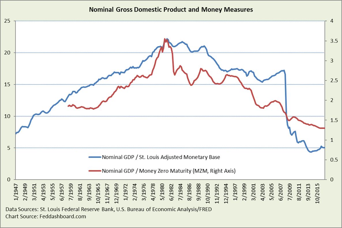 Another view is that the “M” (money supply) used in the formula is narrower than money used in daily life, including consumer credit cards and global financial markets enabled by the global tech and trade transformation, and regulation.
How did the global tech and trade transformation complicate central banking?
Short answer: It smoothed flavors of money and enabled an autonomous financial sector
Since the 1980s, automation and regulatory changes enabled complex financial products, the financial sector has become increasingly autonomous – trading with itself. Outside of times of stress when cash, gold, and regulatory reserves matter most, these new financial instruments (including credit) are closer substitutes for cash than generally realized. Consider one example…
Below, the ratio (blue line) of total financial assets to Gross Domestic Product (GDP) more than doubles from the stability before 1980 to present. At the same time, the change in product prices (red and green lines) is decreasing. Since the mid-1990s, this measure of money has been increasing while prices of tangible products have been moderating.
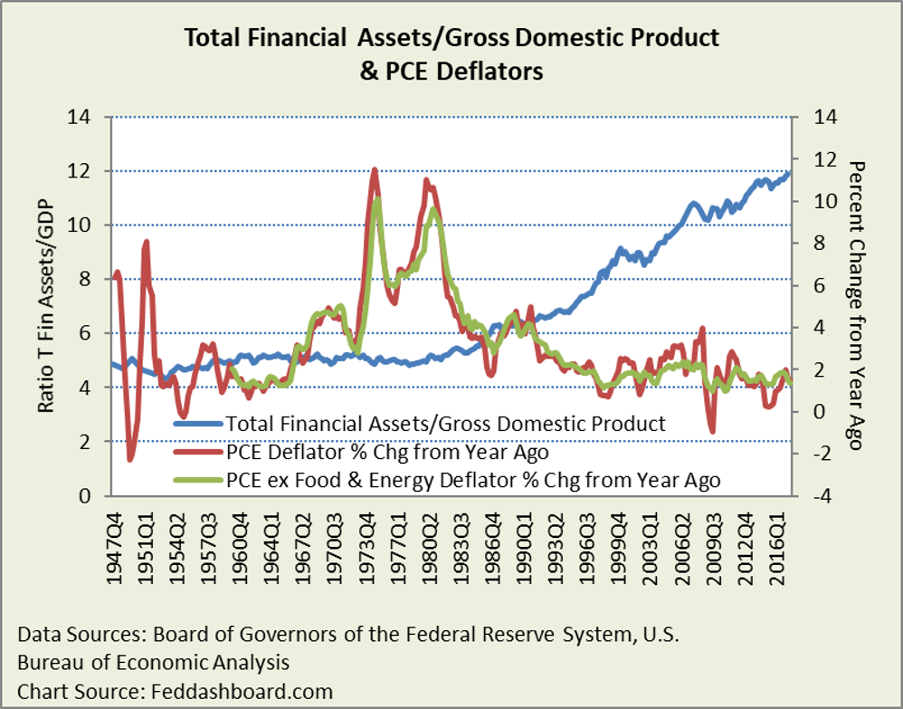 This helps explain why QE didn’t explode product prices — money was already abundant.
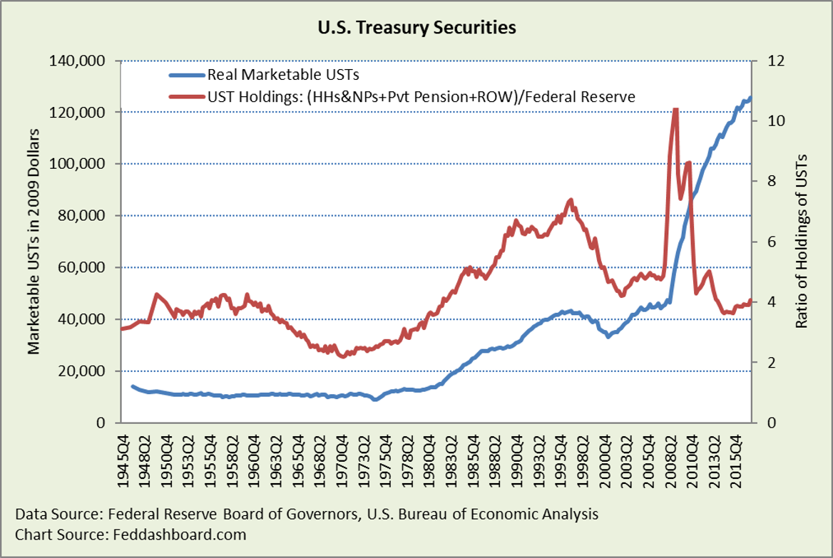
Below is the historical pattern of today’s top holders of U.S. Treasuries (USTs) – households and nonprofits, private pension funds and rest of the world. Top holders have changed over the years. In 1945, banks were by far the top holder.
The Fed went from holding just under 15% from 1945-62, then steadily rose to 30% in 1974, then fell to 11% in 1990 where it held until 1997 before rising to about 18% until 2007 when it dipped as low as 8% in 2009 until returning to the 18% range about 2013.
 Two points:
- There are many buyers of government debt. Central banks aren’t the primary check on government spending, even for higher credit risk countries.
- Today is different from the 1970s. Back then, product price increases were higher, debt-to-income lower, demographics were younger, total financial assets/GDP much lower, Ginnie Mae issued its first Mortgage-Backed Security in 1970, tech and trade transformation was in its infancy, and goods hadn’t yet tipped into relative abundance in the mid-1990s.
Autonomous financial sector creating money on its own and UST holdings beyond the Fed add to the tangible product tech, trade, shopping, and government reasons why the impact of money supply on product prices is less than in the 1970s.
What can central bank tools achieve?
First, QE can bubble financial assets. And, attract other funds flow – most notably funds from the rest of the world and Exchange Traded Funds as we discussed previously in “How to get over 90% of your returns with less stress – start with macro.”
Second, the Federal Funds rate can move tightly-linked private lending rates, such as for credit cards.
Third, monetary policy can lower currency value to make exports cheaper and imports more expensive – import inflation. Thus, it’s a path to both more domestic production for export and increasing inflation. The problem is that a central bank can only control their half of the equation. The European Central Bank (ECB) painfully learned this lesson after working hard to lower the value of the Euro through QE. Then, after the Brexit vote, the Euro/Great Britain Pound rate was back to its late-2009-early-2010 level.
Below, we see consumer goods prices deflected a bit by the Real Trade-Weighted U.S. Dollar Index against seven major currencies.
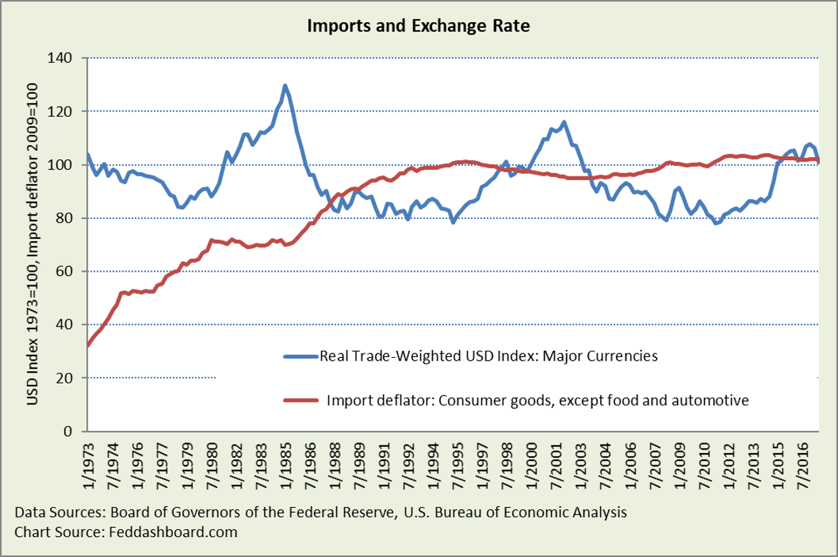 Consumer durables except food and autos have had little price change since the mid-1990s. This frustrates the FOMC. An FOMC desperately seeking inflation can find help in commodities, especially foods, feeds and beverages because that category has grown relative to all goods imports.
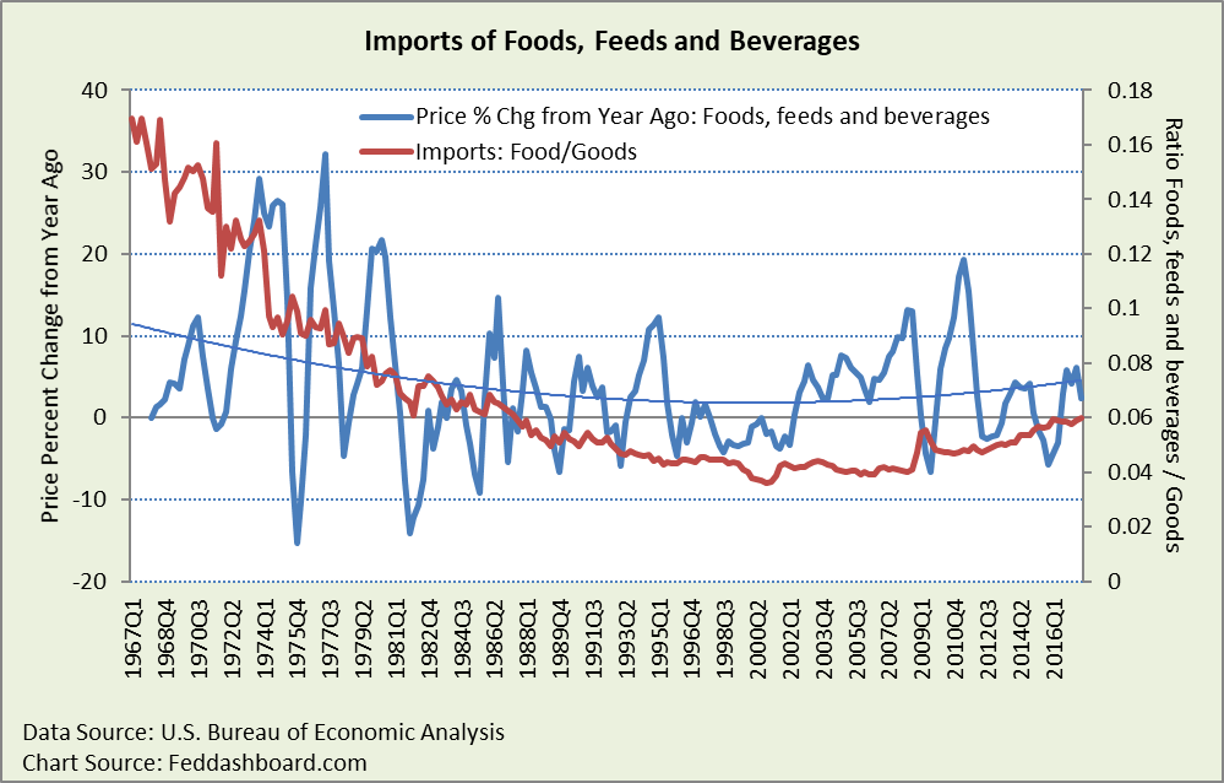 Bad news for the FOMC is that current price increases aren’t as high as the 2002-12 period. Good news is that price increases have been trending up since about 2000.
Investors can watch for signs of price increase:
- Imports of commodity materials and foods. While watching, look for technology and management techniques reducing costs as they have for oil extraction.
- Export growth that strains production resources. While watching, note that the attractiveness of U.S. production is bounded by exchange rates, excess capacity, speed of creating new capacity, costs in other jurisdictions, trade regulations, recent tax changes, and
Fourth, influence bank lending through the interest rate paid on the reserves that banks deposit at a central bank above the amount the required by regulation (Interest on Excess Reserves, IOER). The FOMC’s view has been that the IOER rate needs to be at the high end of the Federal Funds range to achieve the Federal Funds rate target. As of the December 2017 FOMC meeting, 1.5%. The retort is that paying this rate reduces the incentive for banks to lend and the U.S. would be better following the example of Canada and the UK. For more, George Selgin has described these dynamics in a series of articles at the Alt-M blog.
In short, monetary policy works best where it is most direct and not conflicted by global funds flows, other government policy, or other nations.
What does this mean for setting an inflation target?
First, global financial markets make it more difficult to set a target when 1) global financial flows put pressure on an interest rate objective (like defending an exchange rate) and 2) global markets enable wealthier investors to circumvent central banks.
Second, product prices fanning out on divergent trajectories (rather than clinging together) create two problems:
- Removes the bull’s eye of a true statistical mean to target
- Fosters potential for misallocation, distortion, and inequities as described in “Investors: avoid the theory trap, change how you watch inflation” and further in “How the Fed’s 2% target created their inflation trap and hurt our growth”
Third, financial stability is impaired simply because of the cross-currents hitting financial institutions and investors as they seek returns. This includes today’s inflation in financial assets versus restrained prices for tangible products.
When a central bank targets an interest rate (again, such as the Federal Funds rate) it’s in pursuit of objectives, such as “inflation” (practically, the core PCE deflator that includes non-monetary causes of price changes), output (Gross Domestic Product), Final Sales to Domestic Purchasers, or unemployment rate.
- The problem is that moving that rate moves more than the intended objectives, resulting in winners and losers
- Thus, the real question may be whether the Fed’s price stability objective should focus on minimizing distortions
Insight from history
- In his General Theory (1936), John Maynard Keynes wrote of Alfred Marshall, “It seems that we have been living all these years on a generalisation which held good, by exception, in the years 1880−86, which was the formative period in Marshall’s thought in this matter, but has never once held good in the fifty years since he crystallised it!”
- Today, theory clings to conditions observed statistically around the 1970s. Then change happened. The tipping point was the mid-1990s.
For central bankers, data show it’s time to rethink and break groupthink
- Avoiding distortions to financial asset prices as much as tangible product prices
- Reaching an accord with other policy-makers to avoid conflicts over price policy. For example, governments and private sector seeking to lower health care prices while the FOMC is seeking higher prices. Or, central banks seeking to raise prices while governments are doing structural reform, such as cutting excessive regulation. The recent U.S. tax legislation will be a powerful force not only in tax rates, but also for industry structure change in U.S. and abroad.
- Rethinking central bank tools in a world where 1) inflation is lower, 2) the neutral or natural rate of interest is lower because of both the global glut of funds and fewer funds needed for a given amount of production, as we described previously in “Tech & trade – “must discuss” topics for Jackson Hole”, and 3) aggregate demand is less about traditional money measures
For investors, data demonstrate a central bank wild card
The more central bankers miss the data and dynamics, the more forecasts and FOMC “dot charts” will continue to be systematically wrong.
Thus, investors need to track:
- Data that FOMC members state they are watching
- Broader data that the FOMC should be watching
- How quickly the gap closes
This leads to our next exploration in this series Forecasting “inflation?” – avoid the price-productivity trap.
To learn more about how to apply these insights to your professional portfolio, business or policy initiative, contact “editor” at this URL.
Data Geek Notes:
- For insights on monetary aggregate substitution, see William A. Barnett, “Getting it Wrong: How Faulty Monetary Statistics Undermine the Fed, the Financial System, and the Economy.”
- Final sales to domestic purchasers is equal to GDP minus net exports minus change in private inventories. It is also equal to the sum of PCE, gross private fixed investment, and government consumption expenditures and gross investment.
- St. Louis Federal Reserve Bank’s version of monetary base is adjusted for bank reserve requirements. For more on the value of this measure, see “A Reconstruction of the Federal Reserve Bank of St. Louis Adjusted Monetary Base and Reserves,” by Richard G. Anderson and others at the St. Louis FRB, 2003.
- Money Zero Maturity is calculated by the St. Louis FRB, it is M2 less small-denomination time deposits plus institutional money funds.
- For a helpful view of financial markets and money see “Low Inflation in a World of Securitization,” by Brett W. Fawley and Yi Wen at the St. Louis FRB, 2013.