The global tech and trade transformation has enabled a greater supply of funds in more global markets and lower costs of production – leading to a lower natural interest rate.
Knut Wicksell[i], a pioneering Swedish economist, wrote in 1898 that “There is a certain rate of interest on loans which is neutral in respect to commodity prices, and tends neither to raise nor to lower them. This is necessarily the same as the rate of interest which would be determined by supply and demand if no use were made of money and all lending were effected in the form of capital goods. It comes to much the same thing to describe it as the current value of the natural rate of interest on capital.” Over the years, “natural” and “neutral” have been interchanged, yet there are distinctions.[ii]
The natural rate of interest matters because central bankers use it to guide their interest rate policy decisions. In the U.S., this is the Federal Funds Rate, a risk-free, overnight lending rate. In general, in central banks, these are “policy rates.” [iii]
The danger of a policy rate higher than the natural rate is suppressing growth. The danger of a rate too low is “over-heating” an economy and hurting people seeking interest on safe savings.
Simplifying, but hopefully not simplistically
Models of natural interest rates have two components:
- First, a measure of potential growth in an economy. Generally, either a “production function” (growth of labor productivity times the growth of workforce) or a measure of Potential GDP. “Potential GDP” is a measure of what a country could produce if all resources were fully used in a way that didn’t cause excessive price level increases. Potential GDP can be calculated in several ways. In the U.S., the Congressional Budget Office is the primary publisher.
- Second, a way to show the relationship between the growth measure and the policy rate. This can be a simple average or moving average. It can also be a more elaborate formula including both 1) changes in price level, production output, and interest rates and 2) attempts to filter out “noise.”
Production output (also “production” or “output”) is the quantity made of goods and services (doctor visit, hamburger, or smartphone). It is measured as “Real Gross Domestic Product,” Real GDP. “Real” means adjusted for price-level changes. It is not measured by “nominal GDP” where price and quantity changes are combined.
The basic idea is that growth in goods and services produced (Real GDP) primarily depends on real interest rates — lower rates mean more growth.
For curious people, the natural question about natural rates is, “What else is happening?”
Each assumption is a clue
- If the production function approach is used, then it assumes the share of labor input to production has been stable over decades
- If the Potential GDP approach is used, then it assumes 1) the available capacity (“slack” in econ-speak) has been adequately counted and 2) the relationship between price levels and the official unemployment rate (termed the “Phillips Curve” that we explored previously) isn’t overestimating potential “inflation.”
- It assumes the relationship between interest rate and fixed investment has been stable over time, including little change in cost of fixed investment to produce a given level of output
- While making some allowance for the global “cash glut” highlighted by former Federal Reserve Chairman Bernanke, models – to varying degrees – exclude the breadth of financing types used by businesses.
The “global tech and trade transformation” refers to changes in management technique, technology, and trade. Trade includes offshoring of services, parts production, and energy, as well as trade in finished products. This transformation has been progressing for millennia. The current emphasis starts with durable goods exports from Japan in the early 1970s.
The global tech and trade transformation changed each of the above assumptions:
- Labor share of inputs to production has been on a downward trend since 1961, as we’ve illustrated previously
- Potential GDP excludes much slack because of Cold War-era assumptions. It also limits potential production because of the fear of “inflation” that hasn’t yet happened. We discussed this previously in “Potential GDP is potentially misleading” and “Slack Attack.”
- Updating either of the above approaches leads to a view of higher potential production growth and – if this were the primary force — a higher natural interest rate. But, there’s more to the story…
- The link between the Federal Funds rate and fixed investment is weak as we’ve illustrated previously. A reason is that the Federal Funds rate has little influence in calculations used by businesses for investment decisions, such as net present value.
- Cost of fixed investment has been falling. Yet, government statistical agency estimates of investment don’t fully reflect this because they don’t fully adjust for improved product quality. Thus, it is helpful to look at price-quantity curves of final goods and industry sources of the cost of investment and production.
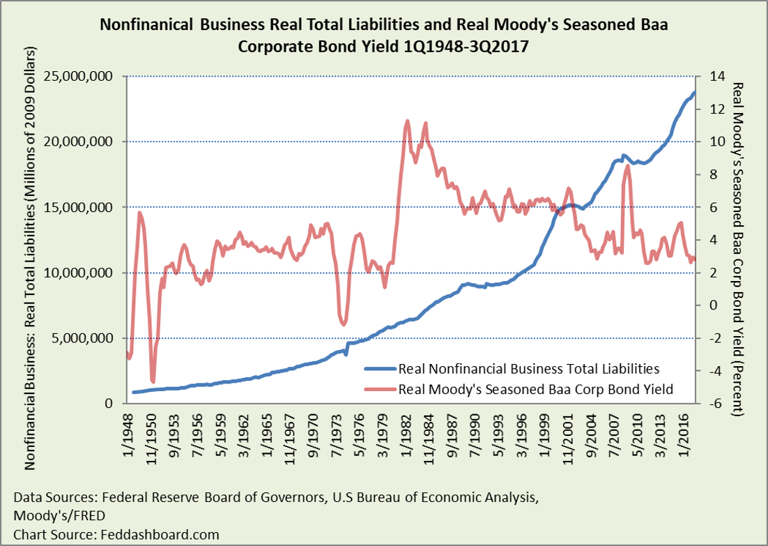
The chart below shows Nonfinancial Business Real Total Liabilities increasing while a common real borrowing rate has been lower since 2001.[iv] This pattern started before 2009, it’s not just about quantitative easing. Lower rates in the face of higher loan demand imply that the supply of funds has been growing faster than demand for funds.
 Nonfinancial Business Total Liabilities compared to Gross Value Added of Nonfinancial Business has grown three-fold from 1959 to 2017.
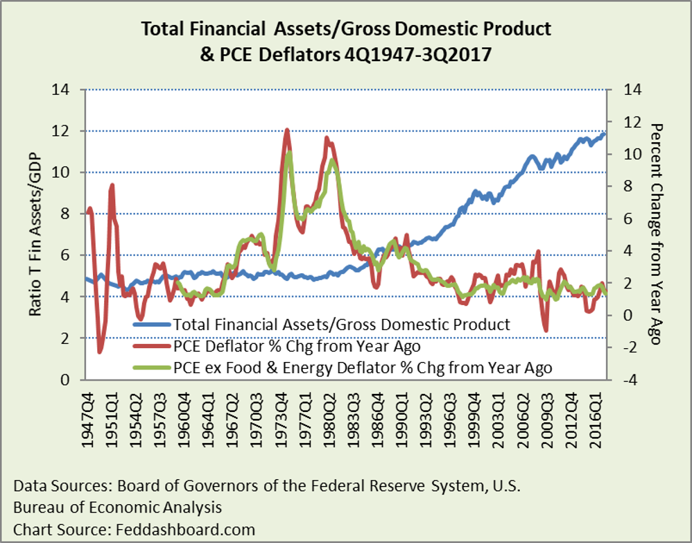
The chart below shows Total Financial Assets compared to GDP has been growing since the 1980s.
This is starkly different from pre-1980s views of a stable ratio of funds to production volume of nonfinancial businesses, such as lending to support fixed investment, inventory and working capital in a manufacturer. Financial businesses have increasingly traded with each other, becoming more autonomous from nonfinancial businesses.
In addition, product price increases have slowed (average of goods prices has been falling since 1995). Lower product prices reflect lower costs of investment and production to make an amount of output. Industry sources of data highlight significant cost reductions – that’s how industry solution vendors make their money, cutting cost for their customers who produce downstream goods and services.
 This chart reflects two more trends:
- Quantitative easing didn’t explode inflation because the system was already awash with funds
- Separation between the financial and “tangible” (goods and nonfinancial services) sectors driven by the global tech and trade transformation. Financial markets have become increasingly global, autonomous from the tangible sector and can circumvent central banks. The tangible sector has lower costs for products that can be traded across distance. Prices that have increased most tend to be for locally-provided services that are more influenced by government regulatory and fiscal policy. A wild card is how a rise of protectionism will affect prices of globally traded products.
Let this settle in…
Data suggest that more funds in more autonomous global markets and lower production cost combined to lower natural interest rates.
Once upon a time, production volume was the primary driver of natural rates. In recent decades, the driver has become funds supply and demand. This is as suggested by Wicksell 120 years ago, but in today’s market structure.
Broader dynamics
Any formula is limited to the variables it includes. Beyond updating basic assumptions, more dynamics are at work…
- Debt/equity ratios have been shifting to improve any financial ratio with equity as a denominator, such as return on equity (ROE). ROE is part of the weighted cost of capital used in the net present value formula for investment decisions. Central bank actions and share-buybacks both contributed.
- Growing global supply of funds flowed from the combination of deregulation, more complex products, more global markets, and more tech. In addition, nonfinancial companies, led by digital tech giants, have increased financial assets as a share of their total assets.
- Global tech and trade transformation means more slack, including global slack bearing on the U.S., digital production slack, and faster provisioning of equipment. Published statistics don’t include all this slack. Further, the notion of “diseconomies of scale” has been melting away for decades as management technique and technology have attacked the causes of diseconomies.
- So-called “headwinds” holding rates down are often a misnomer. The global tech and trade transformation is not like the headwinds of flying west from New York City to Tokyo in a bad week. Instead, it has endured for millennia, other than interruptions from geopolitics and natural disasters.
Insight from clearer data and mechanics
Beginning with business investment “mechanics” helps focus on more relevant government statistics and industry insight, such as required return on investment of a new manufacturing or hospital cost-cutting project.
- Supply of all capital sources (debt, equity, and retained earnings)
- Cost and capacity of nonresidential fixed investment
- Debt loads of businesses and households
- Efficiency of global financial markets. A pulse is in family office investment networks, with wealthy people gaining access to global markets, yet having difficulties finding their preferred investments.
Investor opportunity
- With funds supply higher and demand lower, natural rate naturally falls.
- Understanding the dynamics better than central bankers gives investors an edge. As in sports, they can head to where the ball or puck will be.
Bonus: For econ geeks only
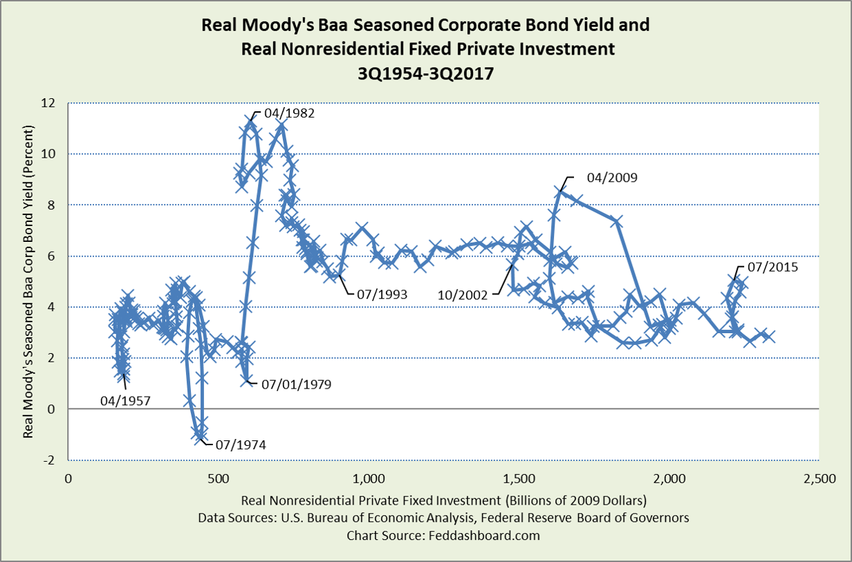
In “Why lower interest rates didn’t create a boom in business investment – 3 reasons might surprise you,” we plotted the Real Effective Federal Funds Rate and Real Private Nonresidential Fixed Investment. Below, this is updated to a business view using the real Moody’s Seasoned Baa Corporate Bond Yield.
 Reaching into the econ recesses of your mind, you might recall the Investment-Savings and Liquidity Preference-Money Supply framework (IS-LM). The IS and LM curves are difficult to determine. Clearer is the quarterly intersections of the IS and LM curves – shown by the “X”’s above.
The 1950s and 60s have some years of stability. From 1984-1993 there is a steep downslope that could be a mostly stable IS curve with growing funds supply shifting the LM curve to the right.
In the mid-1990s, behavior changes – investment mostly just grows, enabled by the global tech and trade transformation:
- Financial markets automation in the late 1980s
- Factory automation and robots in the early 1980s
- Networking in the early 1990s
- Debt increases, especially growing since the 1990s
- Business process automation in the 2000s
- Digitization in the 2010s
In these and other data, our economy changed dramatically in the mid-1990s. This is another reason for a rethink of monetary policy.
To learn more about how to apply these insights to your professional portfolio, business or policy initiative, contact “editor” at this URL.
Data Geek Notes
[i] For a short introduction to Knut Wicksell, see Anderson, Richard G. 2005. “Wicksell’s Natural Rate.” Federal Reserve Bank of St. Louis, Economic SYNOPSES, Number 6.
[ii] For the history of the terms “natural” and “neutral” rates, see Lindhahl, Eric. 1939. Studies in the Theory of Money and Capital.
[iii] For helpful summaries of research in this area, see Laubach, Thomas, and John C. Williams. 2016. “Measuring the Natural Rate of Interest Redux.” Business Economics 51, pp. 257–267. And, Rachel, Lukasz, and Thomas D Smith. 2015. “Secular Drivers of the Global Real Interest Rate.” Bank of England Staff Working Paper 571, December.
[iv] Lukasz and Smith helpfully note that much analysis is with a risk-free government securities rate whereas businesses borrow at higher rates. As shown previously, the Fed Funds rate and corporate bond yields do not have a consistent relationship. The real Moody’s Baa bond yield is calculated after-the-fact by subtracting the 1-year change in the Personal Consumption Expenditures deflator, rather than what people at each point in history would have been guessing about price levels in future years of a bond’s life.

